Array Algebra #

Authors: Taliesin Beynon (contact@tali.link)

Introduction: Array algebra is the theory and practice of manipulating and computing with arrays of numbers. The underlying ideas are quite simple and intuitive, once you’re used to them! This practical will cover some of the core concepts, and focus on visualizing the operations to make them easier to understand.

Topics: numpy, jax, array processing

Learning objectives:

Understand how arrays of number of various sizes and shapes can represent data from the real world
Manipulate these arrays to perform useful computations
Understand how shapes of arrays are transformed by these operations
Detect bugs in existing code
Choose the right transformations to accomplish a given task.

Installation and imports #

## Install and import anything required. Capture hides the output from the cell. 
#@title Install and import required packages. (Run Cell)
import os 
import matplotlib.pyplot as plt
import numpy as np

What are arrays? #

To get started we’ll cover some very basic ideas in array algebra.

A numeric array is a data structure containing numbers. These numbers are organized in a system, grid-like way. We can classify arrays by how they organize these numbers – in particular the shapes of grids they use. But first, let’s introduce some terminology.

Each number in an array lives in a cell. The value of the cell is the number it contains. The position of the cell is where the cell is located within the array.

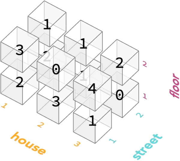
We can make a useful analogy between an array of numbers and a neighborhood of houses. The houses are organized into streets, and each house contains a certain number of people.

A single house #

The simplest kind of neighborhood only has one house in it! This house doesn’t need to have an address, because we don’t need to distinguish it from any other houses. The postman will clearly know which house to go to without an address!

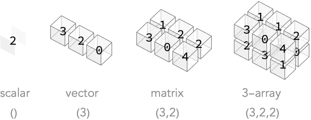
On the left we show this neighborhood, which has only one house that contains 3 people. On the right we show the array it corresponds to in our analogy.

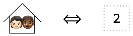
This kind of array is so simple that most people don’t usually call it an array, but is technically a 0-array! More frequently it is known as a scalar.

Here is how we can create such a scalar in numpy. Run this code and see what the shape of this array is, we’ll talk more about this later!

scalar = np.array(3)
scalar.shape

A single road #

Now let’s consider a neighborhood with just one street, and 3 houses on it.

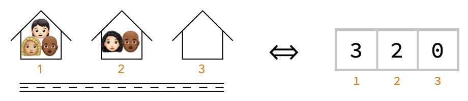
Notice we’ve labeled each house with its street address, just like we’ve labeled each cell with its position in the array on the right.

This kind of array, where a cell position consists of a single number, is called a 1-array, or vector.

Here is how we can create this vector in numpy: run this code and again notice the shape.

vector = np.array([3, 2, 0])
vector.shape

Task: try to guess what shape means from these first two examples

Two streets #

Now let’s imagine a neighborhood with two streets, both with the same number of houses (3) on each.

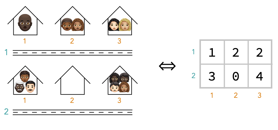
To locate a house in the neighborhood, we need both the street name (1 or 2), and the house number on that street (1, 2 or 3). Similarly, to locate a cell in the array, we need the number of the row (1 or 2), and the number of the column (1, 2, or 3). For example, the cell at address (2, 3) has value 4.

This kind of array, in which the positions of cells require two numbers to describe them, is called a matrix or 2-array. We call these concepts of street name and house number the axes of the matrix.

Here’s how we can create this example in numpy. Again, run this code to see what shape it produces.

matrix = np.array(
	[[1, 2, 2],
 	 [3, 0, 4]]
)
matrix.shape

$Aborted

The following code will look up the value of the cell at address (2, 3), in other words the number of people on the

matrix[1,2]

Notice that we used the position [1,2] rather than the position [2,3] to look up the cell This is because Python uses “zero-indexing”: indices in arrays and lists are counted starting at 0 rather than 1. So the first house has index 0 rather than 1. It’s generally easiest to use ordinary “one-indexing” in one’s head, and then convert these indices to Python’s zero-indexing convention when reading and writing code.

Also notice that the first axis above

Task: Modify the code below to look up the number of people in the top-left house in the neighborhood / the value of the top-left cell in the matrix:

matrix[1,2]

Multi-story houses #

Now let’s imagine that there are two floors in each building in our 2 × 3 neighborhood.

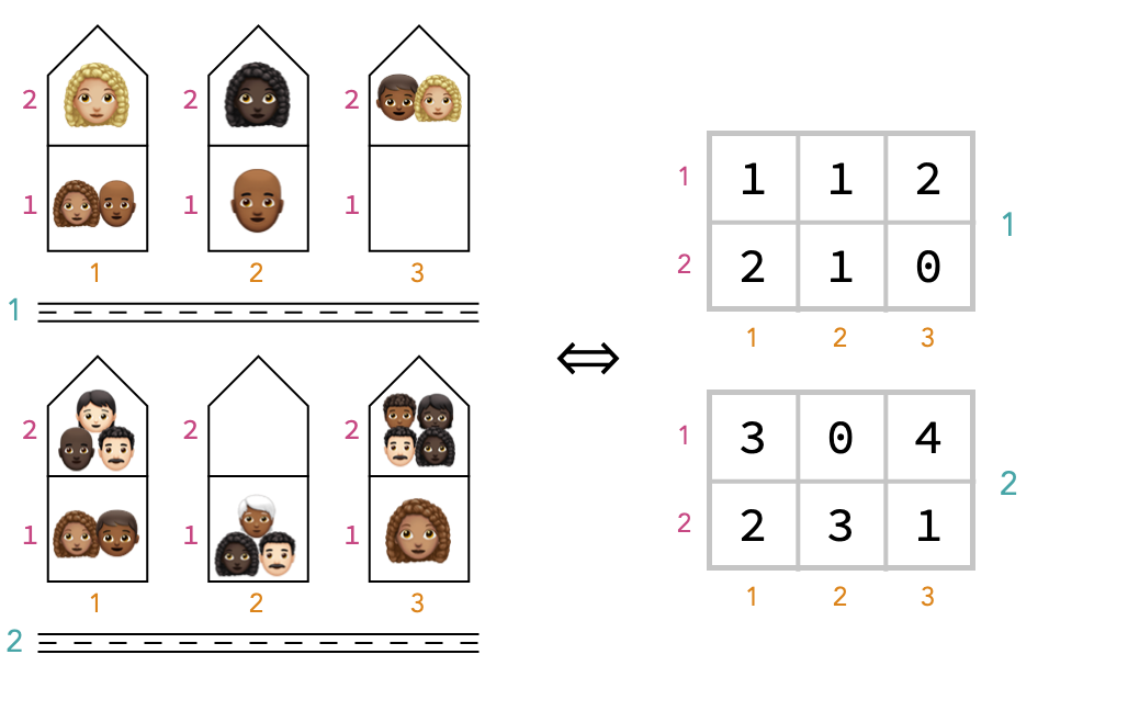
To identify a household, we’ll need the street address (which requires the street name and house number), and an additional floor number.

Similarly, for the array representing this neighbourhood, we’ll need three indices to specify a cell location, one for each of the axes we called street name, house number, and floor number. For that reason, we call this kind of array a 3-array, or tetrix.

We’ve shown it on the right by drawing two matrices on top of one another, but we can also imagine it in 3 dimensions, where we have labeled the axes:

Here’s the numpy to create this array:

matrix = np.array(
	[[[1, 2], [1, 2], [2, 0]],
 	 [[3, 2], [0, 3], [4, 1]]]
)
matrix.shape

Notice that the innermost lists like [4, 1] are describing the people in each house, and so gather together the numbers for the last axis, which is floor axis.

The lists containing these, such as [[3, 2], [0, 3], [4, 1]] are describing the houses in an entire street, and gathers together the values for the second-to-last axis, which is the house number axis.

And the outermost list we passed to np.array is describing all the streets in the neighborhood, and gathers together the values for the first axis, which is the street number axis.

As you can see, when using numpy we have to choose an order for the axes. The array is then representing for input and output purposes as a list of list of … lists, with the outermost lists corresponding to the first axis, and the inner most list corresponding to the last axis. In this example, we’ve chosen the axis order street name, house number, floor number.

Task: modify the code below to create the array using the alternative axis order of floor, street, house. if you’ve got it right, the print statement should then produce the output “4”:

matrix = np.array([
	[[1, 1, 2],
	 [3, 0, 4]],
	[[9, 9, 9],
	 [9, 9, 9]]] # change the 9s
)
print("count of people in house 3 on street 1 on floor 2: ", matrix[1, 0, 2])

Higher order arrays #

We can go climb above the third step of the array ladder quite easily, to 4-arrays, 5-arrays, etc.

For a good analogy, think about a neighborhood in which the houses are apartment buildings which have a fixed number of floors and a fixed number of rooms within each floor. This gives us a 4-array, with the new, fourth axis being room number.

The only requirement for a nested set of data to be an n-array is that the size of each axis is fixed. In our analogy, this is like saying that each street has the same number of houses, each house has the same number of floors, each floor has the same number of rooms, etc.

In case you’re wondering, the “n” in n-array is known as the order of the array. It is also sometimes called the dimensionality of the array.

Named vs positional axes #

We should emphasize at this point that numpy and jax do not allow you to use names like floor, street, or house for axes. Instead, we can only refer to the axes by consecutive integers 0, 1, 2, …, where 0 refers to the first axis, 1 refers to the second axis, etc. Once we pick an ordering for the axes, we must stick to it and remember and document the order we chose.

For example, the cell containing 4 above is conceptually located in the cell (house=3, street=1, floor=2) but numpy does not support specifying array positions in this way, so we must instead locate this cell with the tuple (3,1,2) once we have chosen to use the (house, street, floor) axis ordering.

This lack of named axes is unfortunate, since it makes it harder to tell what is going on, but libraries exist to add axis names and future deep learning frameworks are likely to be built around this feature (see the Tensors Considered Harmful blogpost for much more information about this topic). Often, certain orders of axes are required by libraries – deep learning libraries often require the first dimension to be a batch dimension, for example.

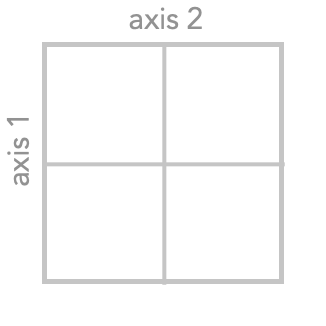
Shapes #

The shape of an array is the description of what the valid cell positions are for that array.

For example, a 4 × 2 matrix, or in other words a 2-array with shape (4,2), contains 8 cells.

Here are the positions of these cells, where we are using 0-indexing for indices:

import itertools
list(itertools.product([0, 1, 2, 3], [0, 1]))

[(0, 0), (0, 1), (1, 0), (1, 1), (2, 0), (2, 1), (3, 0), (3, 1)]

Task: modify the code below to produce the valid positions for our multi-story neighborhood, using the axis order of street name, house number, floor number. you should get a list with 12 positions in it.

list(itertools.product([0], [0], [0]))

Task: modify the code below to produce the valid positions for a 0-array / scalar! you should get a list with exactly one position in it, since a 0-array contains exactly one cell.

list(itertools.product([0], [0], [0]))

Kinds of array #

Let’s summarize the kinds of arrays we’ve just seen in a table, as well as the obvious generalizations:

num of axes	full name	short name	form of shape	num of cells
0	0-array	scalar	()	1
1	1-array	vector	(n)	n
2	2-array	matrix	(n, m)	n × m
3	3-array	tetrix	(n, m, p)	n × m × p
4	4-array		(n, m, p, q)	n × m × p × q
n	n-array		(m₁, …, mₙ)	m₁ × … × mₙ

Here’s a quick gallery of examples of n-arrays of different orders, along with their shapes:

Recap #

We introduced 0-arrays / scalars, 1-arrays / vectors, 2-arrays / matrices, and 3-arrays.

An array is composed of cells. A cell has a value, which is the number it contains, and a position, which is a way to locate the cell within the array.

Each cell’s position is described by indices, one for each axis of the array. An n-array has n distinct such axes.

Each index can be an integer value in the range 0..m-1, where m is the size of the array along that axis. Because Python uses zero indexing, the index zero refers to the first row / column / layer / channel, etc.

The tuple of axis sizes is called the shape of the array. The shape describes the maximum index for each axis.

For a scalar the shape is an empty tuple (), for a vector of m cells it is a singleton tuple (m,), for a matrix of m × n cells it is a pair tuple (m, n), etc.

Working with image arrays #

To get more practical, we’re going to look at a common use-case in deep learning, which is dealing with arrays that represent images.

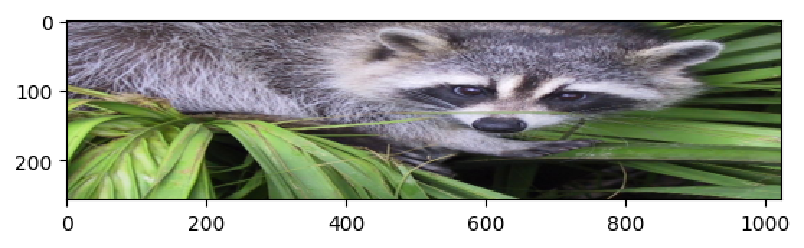
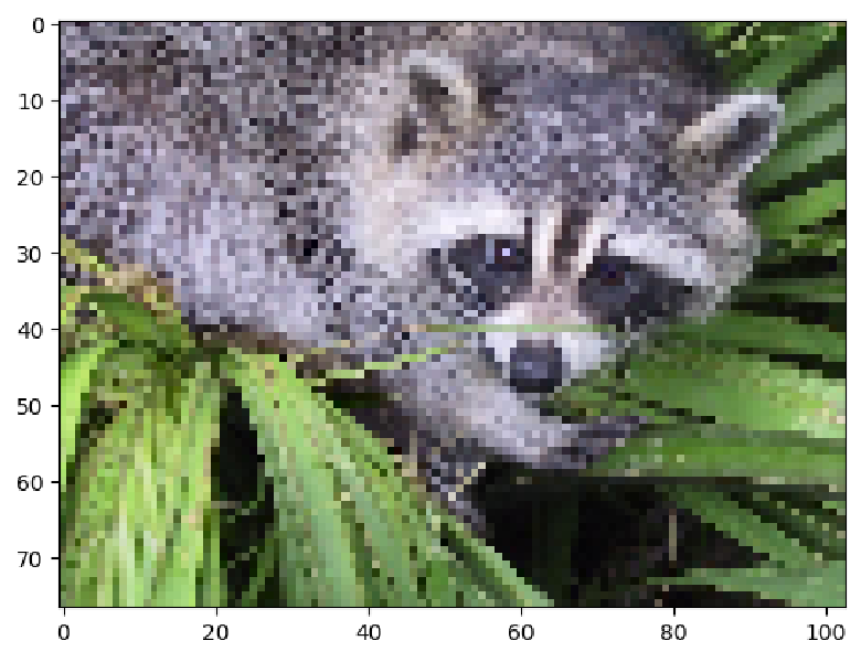
We’ll begin by loading an example image array from the SciPy library:

import scipy.misc
image_array = scipy.misc.face()

As with any array, we can ask what shape it is – how many axes does it have, and what are their sizes?

image_array.shape

(768, 1024, 3)

We can see it has 3 axes, with sizes 768, 1024, and 3. That means the number of cells in the array is 768 × 1024 × 3 = 2,359,296. Each cell in the array contains a number, which we can access by providing the position of the cell. Here’s the number at address 0,0,0, which we look up using the […] syntax:

image_array[0,0,1]

The maximum and minimum values that are present in the entire array can be found with the min and max methods:

(image_array.min(), image_array.max())

(0, 255)

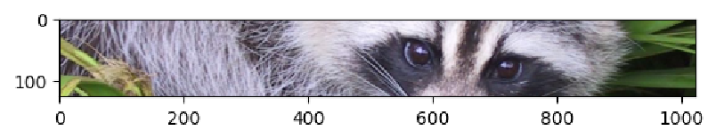
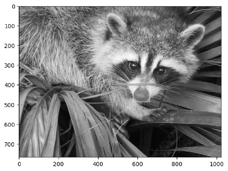
Values in the range 0 … 255 represent the brightness of the image at a particular horizontal and vertical positions – we call this a pixel. Let’s now show this image using the imshow function:

plt.imshow(image_array)

As you can see the horizontal positions range from 0 to 1024, and the vertical positions from 0 to 768. It’s a general convention that the vertical positions by the first axis of the array (the rows), and the horizontal positions are encoded by the second axis of the array (the columns).

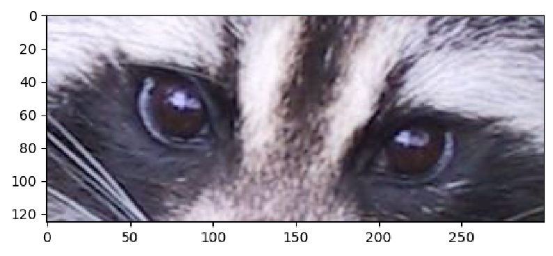
We can demonstrate this by slicing the array along the first axis, so that we take only rows 250 to 375:

sliced_image_array = image_array[250:375]
sliced_image_array.shape

(125, 1024, 3)

Notice there are now only 375 - 250 = 125 rows in this new array. Let’s plot this sliced array. We can see we’ve got an image that shows only a vertical section of the original iamge:

plt.imshow(sliced_image_array)

We can similarly slice the array horizontally. Let’s do both vertical and horizontal slicing. Notice that the vertical slice information is the first argument to […] and the horizontal slice information is the second argument, because the n’th argument is applied to the n’th axis:

sliced_image_array = image_array[250:375, 500:800]
plt.imshow(sliced_image_array)

Task: Modify the code below to display only the nose of the raccoon!

plt.imshow(image_array[250:375, 500:800])

Color channels #

The third axis of these arrays has size 3. This axis represents the color channel. Cells in the first address of this axis represent amounts of red light, cells in the second green light, and cells in the third blue light. Different mixtures of these light amounts produce all the colors a computer screen can display.

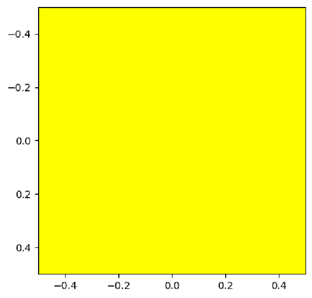
For example, we can form the color yellow as an equal mix of red and green light. Here we demonstrate this by creating a 1 × 1 × 3 array, representing an image containing a single pixel. We fill this array with equal amounts of red and green light:

def plot_color(r, g, b):
  return plt.imshow([[[r,g,b]]])
plot_color(255, 255, 0)

Task: Modify the call to plot_color below to produce a pink image:

plot_color(255, 255, 0)

We will now copy our original image array, and modify it to change some of the pixel values. We’re going to modify the noise of the racoon to be blue. To do this, we’ll set values of part of the array corresponding to the nose.

clown_image_array = image_array.copy()
clown_image_array[420:490, 575:665, 2] = 255
plt.imshow(clown_image_array)

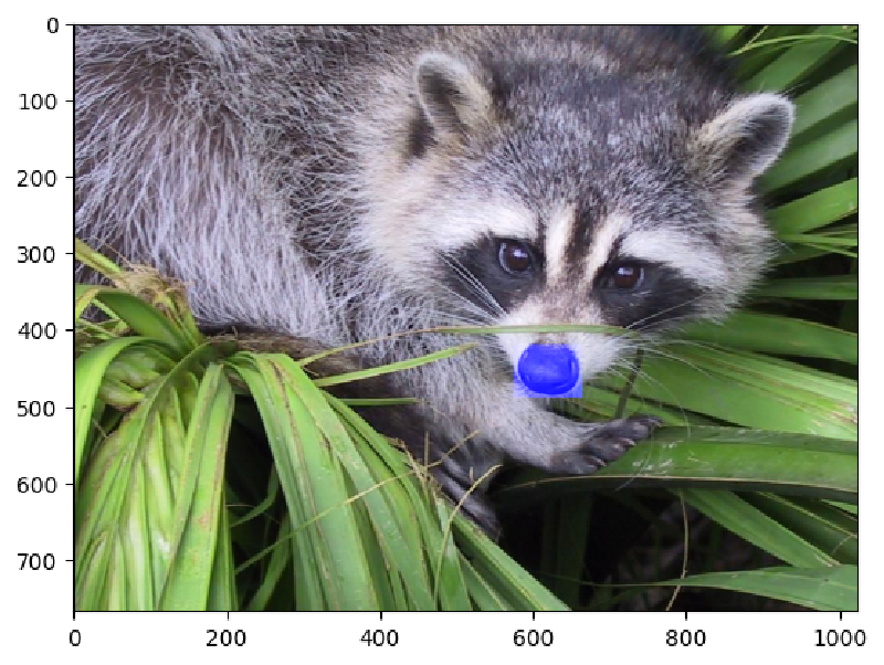
We changed a particular slice of the array, setting it to the maximum value. This slice corresponded to the red channel of a rectangle of pixels around the raccoon’s nose.

Task: It was recently discovered that the raccoon in this image was an important witness in a state investigation into illegal logging. For this reason, we need to protect the identity of the racoon by censoring its eyes. Modify the code below to replace the section around its eyes with a black rectangle.

Hint: to see all color channels to a value rather than just the blue channel, you can use : instead of 2.

witness_protection_array = image_array.copy()
witness_protection_array[420:490, 575:665, 2] = 255
plt.imshow(witness_protection_array)

Tinting an image #

We can modify the amounts of color in the racoon array by multiplying the color channels with a 1 × 1 × 3 array that represents the factor with which to multiply each channel. Let’s double the brightness of the blue channel, and keep the other channels the same:

plt.imshow(clown_image_array * np.array([[[1, 1, 2]]]))

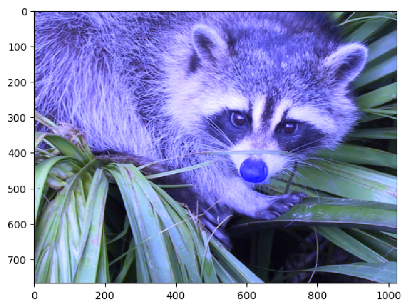
We received a warning because the brightness values of the blue channel now exceeds 255, which is the maximum amount of brightness that can be displayed. These >255 values will still be intepreted as 255 for plotting purposes. Notice also that the color of the green leaves didn’t change much, because they don’t have much blue light in them to begin with!

Task: Modify the code below to multiply the green channel by a factor of 2 instead of the blue channel:

plt.imshow(clown_image_array * np.array([[[1, 1, 2]]]))

Grayscale images #

We’ve seen that images with three color channels are color images, with the color channel corresponding to the $3^{\textrm{rd}}$ axis of the array. If an image array does not have a $3^{\textrm{rd}}$ axis, then we do not have color information, and we call this a grayscale image.

Let’s extract only the green color channel of our racoon using slice notation […] to obtain a grayscale image:

def plot_grayscale(array):
  return plt.imshow(array, cmap='binary_r')
plot_grayscale(clown_image_array[:, :, 1])

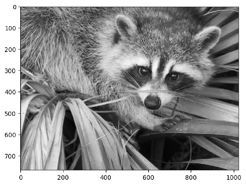
The slice [:, :, 1] requested all rows and all columns of the original array, but only the second (green) color channel.

Task: Modify the code below to plot the blue color chanel of the original image as a grayscale image. You should see that the leaves are darker in the grayscale image derived from the blue color channel than the grayscale image derived from the green color channel, because of course leaves reflect mostly green light! The nose of the raccoon should appear bright white, since we set it’s blue channel to have the maximum value earlier.

plot_grayscale(clown_image_array[:, :, 2])

How do we obtain a single grayscale image that incorporates the brightness values from all three color channels, rather than taking only one at a time?

To do this, we want to total amount of light at a given position in the image, irrespective of whether it is red, green, or blue light. Therefore, we wish to sum over the third axis – the color channel axis. Recall that axes, like most things in Python, start counting at 0, so the third axis corresponds to axis=2.

plot_grayscale(clown_image_array.sum(axis=2))

When taking photographs with old-fashioned cameras, it is important to know the total amount of light that is coming into the camera’s lens, so that we can set the exposure correctly.

We’ll now do a similar thing with our image. We wish to find the average amount of light that is present in the image. To do this, we wish wish to average over the horizontal and vertical and color channel axes. We’ll use the mean method to do this:

image_array.mean(axis=(0,1,2))

110.16274388631184

Task: Modify the code below to calculuate the average amount of light in the clownified raccoon image. Before you evaluate the code, predict whether this mean value should be larger or smaller than the mean value above, and by roughly how much.

image_array.mean(axis=(0,1,2))

We can also calculate the average color of an image. To do this, we will simply avoid summing over the color channel, so that we get an average green, average blue, and average red amount of light that we can then interpret as an average color. Run the code below:

image_array.mean(axis=(0,1))

array([110.67604192, 117.72977066, 102.08241908])

Task: Modify the call to plot_color below to visualize the average color that you computed above. It should appear slightly green, because the image consists of mostly green leaves and a mostly black-and-white raccoon:

plot_color(0, 0, 0)

Slicing #

In the previous section, we dealt with an color image array, a 3-array representing the pixels of an image.

The first two axes were spatial: the first axis represented the vertical and second axis the horizontal arrangement of pixels. The sizes of these axes corresponded to the number of pixels in the vertical and horizontal directions of the image.

The third axis of an image array is quite different, since it represents color, with the size of this axis being 3 because there are 3 color channels that, when mixed together, allow us to display most of the colors that are visible to humans. The indices that are usually used for color channels are 0 ⇔ red, 1 ⇔ green, and 2 ⇔ blue. This kind of axis is sometimes called a discrete axis, since the particular integers or order of cells in this axis isn’t important – we can rearrange the order of colors (red, green, blue) any way we like as long as all our code is changed to match the new convention.

In this section, we’re going to be a little more explicit with slicing, and take you through some detailed examples.

Let’s play with a simple image that illustrates this. It will be a 5 × 4 color image that depicts a red capital letter “F”, with an aquamarine colon after it. Since images are stored with the color channel as the last dimension, we will choose to build the require image array by using the dstack function in numpy to represent the three color channels separately, which makes the data easier to read.

f_array_r = np.array(
[[1,1,1,0],
 [1,0,0,0],
 [1,1,0,0],
 [1,0,0,0],
 [1,0,0,0]])
 
f_array_gb = np.array(
[[0,0,0,0],
 [0,0,0,0],
 [0,0,0,1],
 [0,0,0,0],
 [0,0,0,1]]
)

f_array = np.dstack((f_array_r, f_array_gb, f_array_gb))
plt.imshow(f_array * 255)

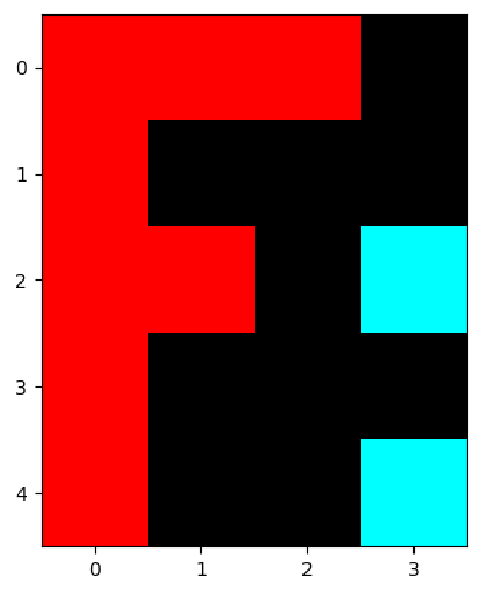
The image array is a 5 × 4 × 3 array, since it is 5 pixels high, 4 pixels wide, and has 3 color channels:

f_array.shape

(5, 4, 3)

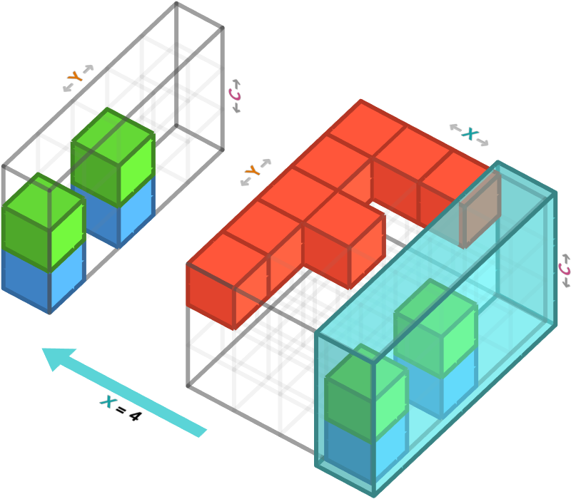
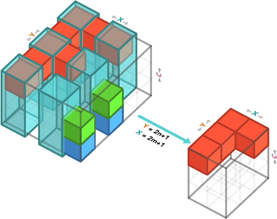
We can visualize this 3-array using a 3 dimensional cube diagram like before, where each cube represents a cell of the image array. Here we will draw the cube as solid if the value of cell is 1, and as empty if the value of the cell is 0. We will also draw cells that live in the red color channel in red, cells in the green channel in green, etc.

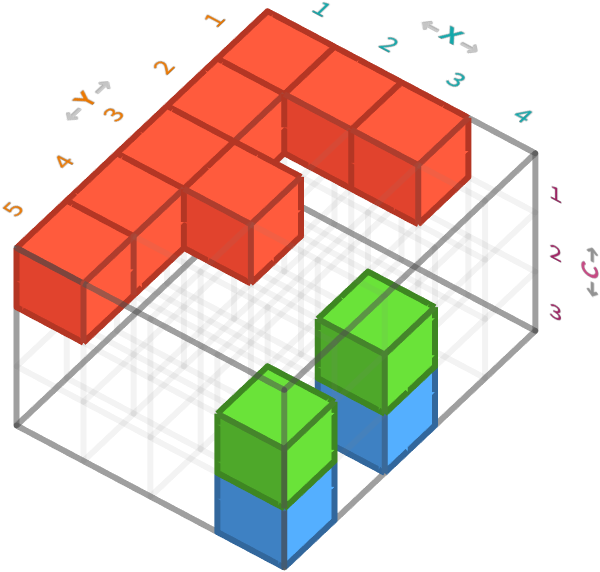
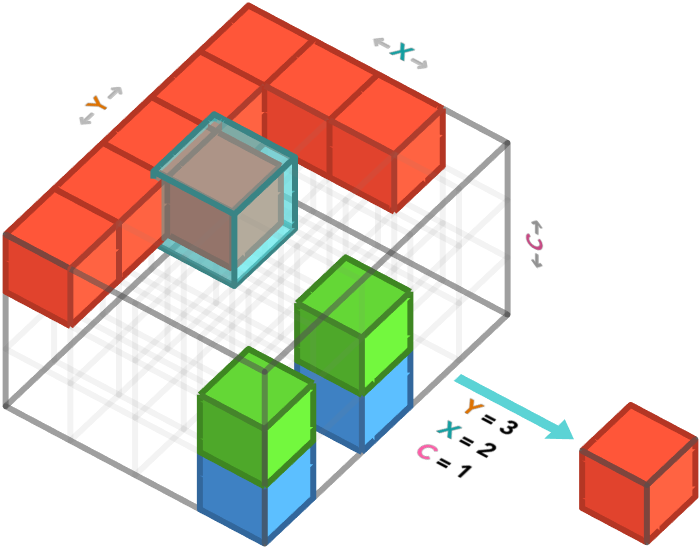
The axis order for this image array is rows (Y), columns (X), and color channels (C).

Specifying one axis #

The first kind of slicing we will do is just to specify an index for a specific, single axis in the 3-array. This will select all cells that have that index. The result will be a 2-array whose axes are the ones we did not specify. Let’s look at an example.

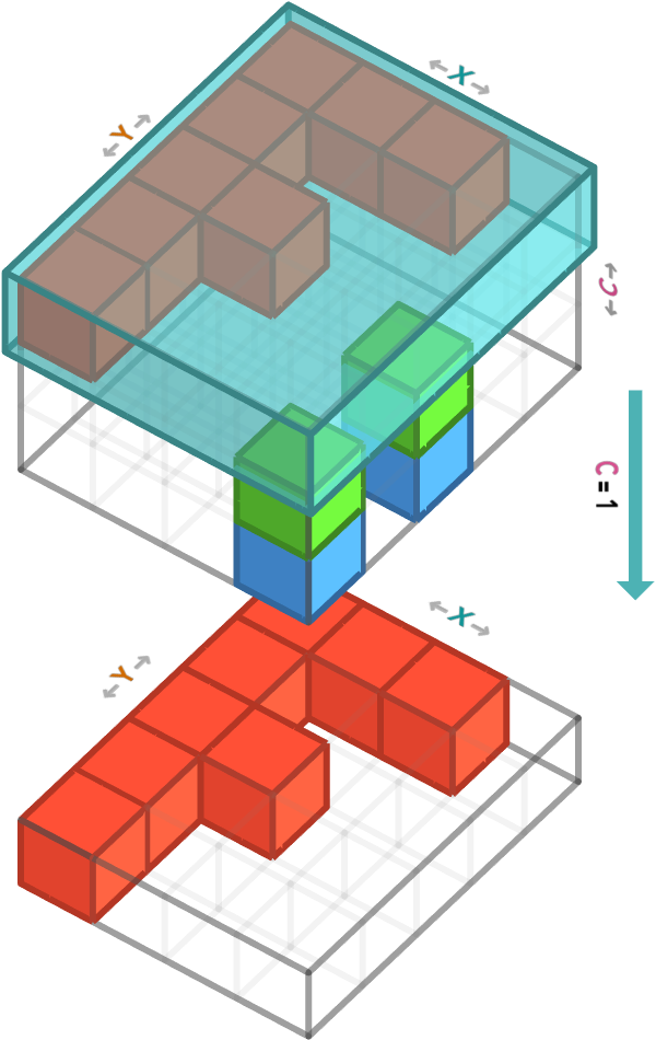
Let’s specify the first axis, which is the rows axis. If we select the third row from the 5 × 4 × 3 sized 3-array, we obtain a 4 × 3 sized matrix whose axes correspond to the columns and color channels:

We can perform this operation in numpy using by specifying the row we want in the first position of the slice [...] notation, and specifying the other axes as :, which means take all indices in that axis. Here we are selecting the third row, which is indexed as 2 in Python:

f_array[2, :, :]

array([[1, 0, 1],
       [1, 0, 1],
       [0, 0, 0],
       [0, 1, 0]])

Task: Explain why the pattern of 0s and 1s in the above array corresponds to the slice shown in the cube diagram above. Hint: notice there are 5 solid cubes in the diagram, and 5 1’s in the array.

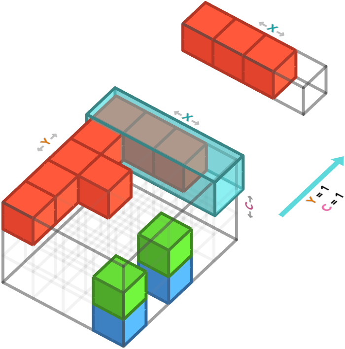
Similarly, if we slice a particular column from this 3-array, we obtain a 4 × 3 matrix (aka 2-array) whose axes correspond to the rows and color channels. Here we select the pixels with X position 4, or if you prefer we are selecting the 4th column.

Since the axis order rows (Y), columns (X), and color channels (C), we must select the second axis to have index 3 (meaning fourth).

f_array[:, 3, :]

array([[0, 0, 0],
       [0, 0, 0],
       [0, 1, 0],
       [0, 0, 0],
       [0, 1, 0]])

Task: Again, explain why the pattern of 0s and 1s in the above array corresponds to the slice shown in the cube diagram above.

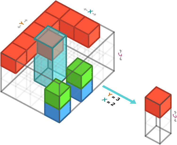
If we slice a particular channel from this 3-array, we obtain a 3 × 3 matrix (aka 2-array) whose axes correspond to rows and columns. Here we take the red color channel:

Since the axis order is rows (Y), columns (X), and color channels (C), we must select the second axis to have index 3 (meaning fourth).

In numpy, this is select that last axis (color channels) to have index 0 (the first channel, red):

f_array[:, :, 0]

array([[0, 1, 1, 1],
       [0, 1, 0, 0],
       [0, 1, 1, 0],
       [0, 1, 0, 0],
       [0, 1, 0, 0]])

Task: Modify the code below to obtain the matrix corresponding to the green color channel. Predict before you run the code what the output will be.

f_array[:, :, 0]

Specifying two axes #

We can also produce a single vector (aka 1-array) by specifying both a particular row and a particular color channel. This leaves only the columns axis unspecified, meaning the result has just this one axis, and is hence a 1-array.

In numpy, we are selecting the first channel (third axis) of the first row (first axis) of pixels:

f_array[0, :, 0]

array([0, 1, 1, 1])

Task: Modify the code below to obtain the vector corresponding to green color channel for the second-to-last row of the image. Predict before you run the code what the output will be.

f_array[0, :, 0]

There are two other combinations of axis we can slice: row and column (which leaves color channel unsliced), and column and color channel (which leaves row unsliced). Let’s examine slicing the row and column:

This corresponds to taking a single pixel from the image, since we are left only with color information.

In numpy, we are specifying a value for the row ($1^{\textrm{st}}$ axis) and column ($2^{\textrm{nd}}$ axis):

f_array[2, 2, :]

array([1, 0, 1])

Task: Modify the code below to obtain the vector corresponding to colors for the bottom-right pixel of the image. Predict before you run the code what the output will be.

f_array[2, 2, :]

Specifying three axes #

Lastly, we can specify all three axis. This corresponds to taking the value of a color channel for a single pixel. After we specify all the axes, there are no axes left, and so we obtain a scalar value. This is effectively a 0-array, an array with no axes, and hence only one possible cell.

In numpy, we are specifying a value for the row ($1^{\textrm{st}}$ axis) and column ($2^{\textrm{nd}}$ axis) and channel ($3^{\textrm{rd}}$ axis):

f_array[2, 1, 0]

Task: Modify the code below to obtain the value corresponding to the blue channel of the top, left pixel. Predict before you run the code what the output will be.

f_array[2, 1, 0]

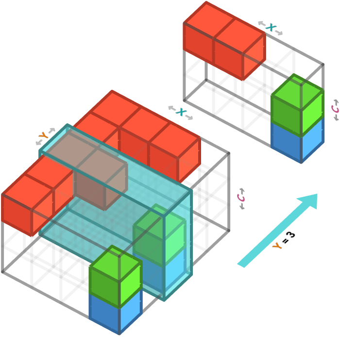
Sub-arrays #

As we saw earlier, we are not limited to specifying a single index for an axis. We can also specify a range of indices. By doing this, we do not remove that axis from the result, since there are now multiple cells within that range on that axis.

Let’s take the first three Y positions, last three X positions, and first two colors channels (red and green):

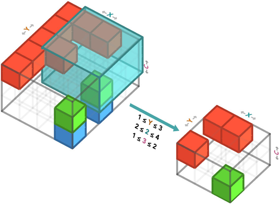
In numpy, we achieve this using the notation start:stop. Note that the start is inclusive, but the stop is exclusive, so 1:4 means taking indices 1,2,3:

f_array[0:3, 1:4, 0:2]

array([[[1, 0],
        [1, 0],
        [0, 0]],

       [[0, 0],
        [0, 0],
        [0, 0]],

       [[1, 0],
        [0, 0],
        [0, 1]]])

This array is a little hard to read, so we will slice the resulting 3-array into two 2-arrays, one for the red and one for the green channels, to print them more easily:

result = f_array[0:3, 1:4, 0:2]
print("red:\n", result[:, :, 0])
print("green:\n", result[:, :, 1])

You might have noticed we’ve been using the syntax : to mean take the entire range from beginning to end – if either start of stop is left off, the meaning is to start / stop at the beginning / end of that axis.

Task: Predict the shape of the array that is produced by the code below. After you’ve done that, predict the values that will be produced, and explain in words what you are doing. Then check your answer by running the code!

f_array[2, 0:3, 2]

array([1, 1, 0])

Step size #

A final variation on slicing is to allow for a “skip” over elements. We can do this using the syntax start:stop:n, which means to take every n’th element, e.g. the values (start,start+n,start+2n, ...) until we go past stop. This n is called the step size.

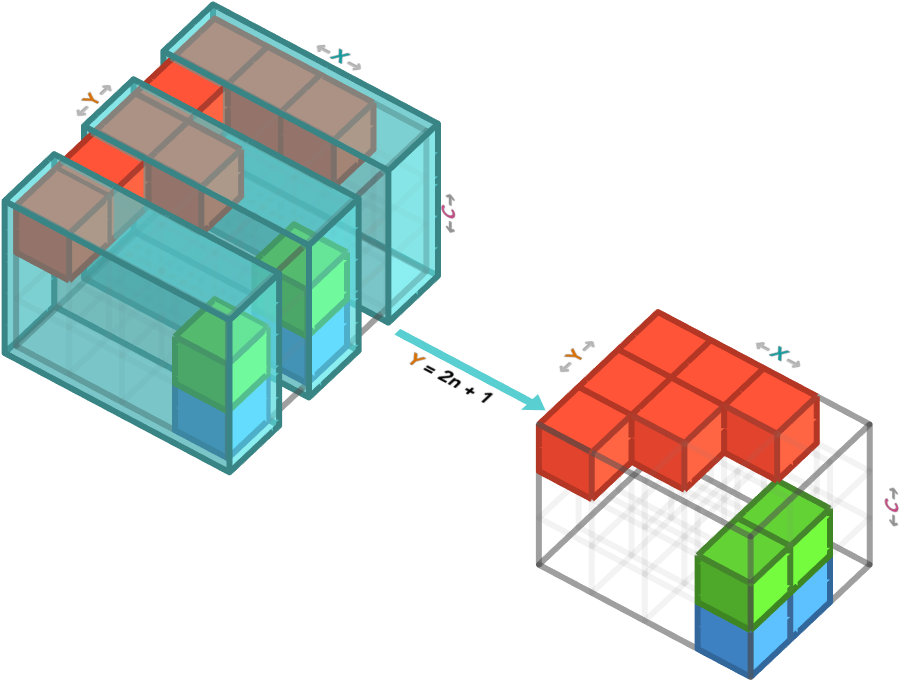
This is particularly useful for subsampling, which is what we do when we want to bring a large data set down to more managable size, and we don’t mind throwing away some of the data to do this. A morbid analogy for this was the ancient process of decimation that was used to punish Roman troops: every company of ten soldiers was forced to execute one of their members. Pretty grim stuff so let’s rather look at what when we step over the Y axis in our cute image of a racoon, taking every third row:

subsampled_image = image_array[::3, :, :]
plt.imshow(subsampled_image)

Our poor racoon was squared vertically. Let’s restore his cute aspect ratio again. To do this we’ll also step in the X axis:

We’ll now take every 10th pixel, so that it is easier to tell that we’ve obtained a lower-resolution image:

subsampled_image = image_array[::10, ::10, :]
plt.imshow(subsampled_image)

Task: for an image of size m × n pixels, and a step size of d, write down the number of pixels the resulting sliced image will have. advanced problem: what step size should we pick to obtain a result with a maximum of d pixels? try to write a Python function that returns this step size.

Transposing #

An operation that you will frequently encounter in dealing with arrays is called transpose. Transpose is the trickiest operation for many people to master, and this is because it exposes one of the flaws of current deep learning frameworks. This flaw is that they today’s frameworks do not use names for axes, and instead store the axes in a fixed order that you as a programmer must keep track of yourself. If axes had names, then you as a programmer would not need to think about the order of axes; any important array operations, like aggregations, slicings, etc, could be expressed purely in terms of axes they affect. This would make array programs much easier to maintain, change, and debug. And the transpose operation would simply not exist at all!

Unfortunately, unnamed axes are still common, and so we will have to deal with them. The first problem is that many operations treat particular axes specially. For example, the first axis is often treated differently from the rest (many operations can “thread” over batches that are taken as the first dimension). The second problem is that operations that combine two or more arrays require their axes to match: the first axis of the first array must match the first axis of the second array, etc. Because of this, you will often have to switch the order of axes in an array so that certain axes end up in certain positions in the axis order.

Transposing matrices #

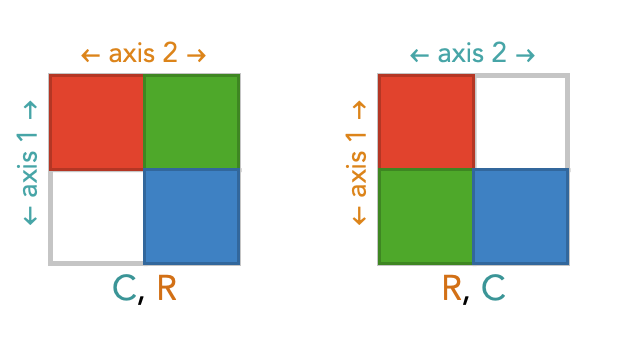
We’ll start with the simplest example, which is that of matrices (2-arrays).

There are two ways we can order the axes of a 2-array: as rows, columns, or as columns, rows.

Here we show square diagrams of the same underlying array, but with these two different orderings of their axes. The red, green and blue colors are placeholders for numbers – we don’t particular care about what the numbers are in this section, instead we want to focus on how transpose changes the order of the axes.

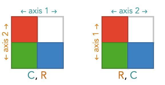
We’ll refer to the axis order below, where the vertical axis is first and horizontal access, as the standard orientation. Notice that the diagram labeled C, R above is not in the standard orientation, but the second diagram R, C is in the standard orientation.

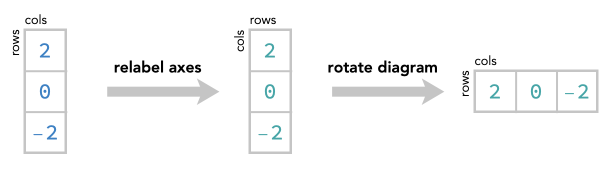
However, we can bring the C, R diagram into standard orientation by “flipping” the entire diagram around its diagonal – to do this you are effectively rotating it in the $3^{\textrm{rd}}$ dimension, like picking up a piece of paper and turning it face down. This has the effect of swapping the two axes of the diagram:

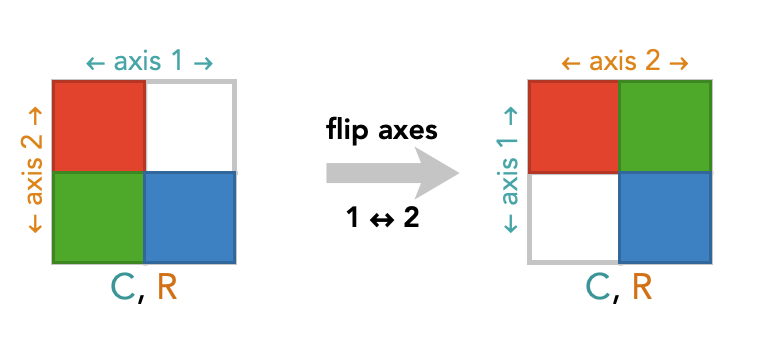
By doing this we are just drawing this oriented square diagram in a different way – we have not changing the contents of the array or the ordering of the axes at all.

By standardizing the orientations, we can see that choosing a different axis order amounts to simply rotating the entire diagram around its diagonal.

Transposing tetrices #

Let’s repeat this exercise for an image array. We’ll look at a very simple 3 × 3 image array, shown below:

cubic_array_r = np.array(
[[0,0,0],
 [0,0,1],
 [0,1,1]])
 
cubic_array_g = np.array(
[[0,1,1],
 [0,0,1],
 [0,0,0]])
 
cubic_array_b = np.array(
[[1,1,0],
 [1,0,0],
 [0,0,0]])
 
cubic_array = np.dstack((cubic_array_r, cubic_array_g, cubic_array_b))
plt.imshow(cubic_array * 255)

This time we’re going to draw cube diabrams in which we label the axes with numbers indicating the position of that axis in a particular axis order. We’ll call these oriented cube diagrams. We’ll still color the axis labels to remind us what these axes represent in the image: rows (Y), columns (X), color channels (C).

Here’s the oriented cube diagram for the standard image array order of rows, columns, color channels:

But there are other ways we could choose to order these axes. Let’s show all 6 oriented cube diagrams for image arrays. The top-left one is the standard one.

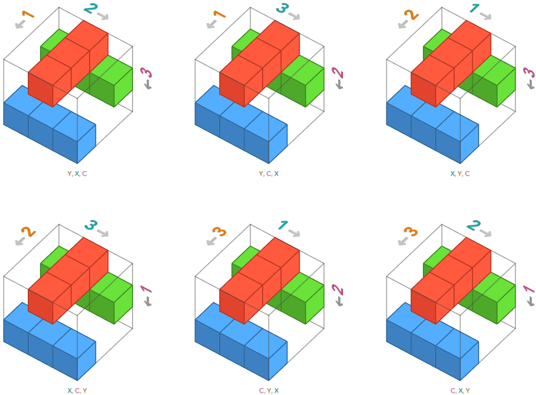
These all depict the same underlying image, but each has a unique representation in numpy. For example, the bottom right array uses the axis ordering color channels (C), rows (R), columns (C). We construct this particular orientation of array by providing the red, green, and blue channels as 3 × 3 matrices for the inner lists:

np.array([
[[0,1,0],  # \
 [0,1,0],  #  |-- red channel
 [0,1,0]], # / 
 
[[1,1,1],  # \
 [0,0,0],  # |-- green channel
 [0,0,0]], # /
 
[[0,0,0],  # \
 [0,0,0],  #  |-- blue channel
 [1,1,1]]  # /
])

Task: explain to your neighbor the connection between the list of matrices above and the cube diagram in the bottom-right axis ordering.

Task: modify the code below to construct the array that uses axis ordering color channels (C), columns (C), rows (R)

np.array([
  ... ,
  ... ,
  ...
])

Transpose as rotations #

This geometric picture provides us for a way to understand what transposes actually are, conceptually.

Here’s how to do this: we adopt a particular convention about how to draw an oriented cube diagram, which is that we should always orient the axes as follows:

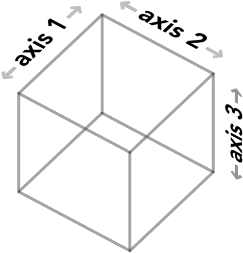
We’ll call a cube diagram shown in this way as being in standard orientation**.**

Not, to actually put an oriented cube diagram in standard orientation we might have to rotate / reflect a cube diagram in three dimensions! For example, the oriented cube diagram for axis order columns (X), rows (Y), color channels (C) must be rotated as follows to put it in standard orientation:

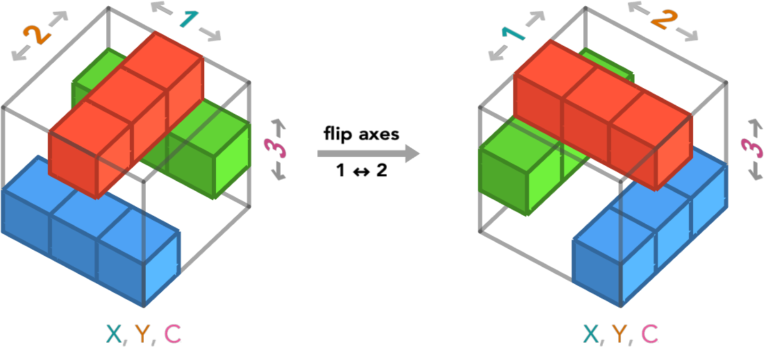
Remember, these two oriented cube diagrams depict the same numpy array with the same axis order. The only difference is that we changed our perspective so that the first, second, and third axes were in standard orientation. We’re only changing how we are visualizing this array.

Here’s how all of the 6 axis orders look when draw them in standard orientation:

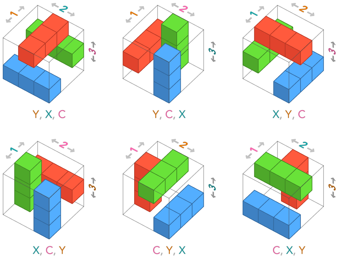
Advanced remark: If you have a pure mathematics background, these 6 elements are the elements of the dihedral group of order 6, which are the isotropies of a triangle. The orientations of higher-order arrays correspond to isotropies of higher-dimensional simplexes.

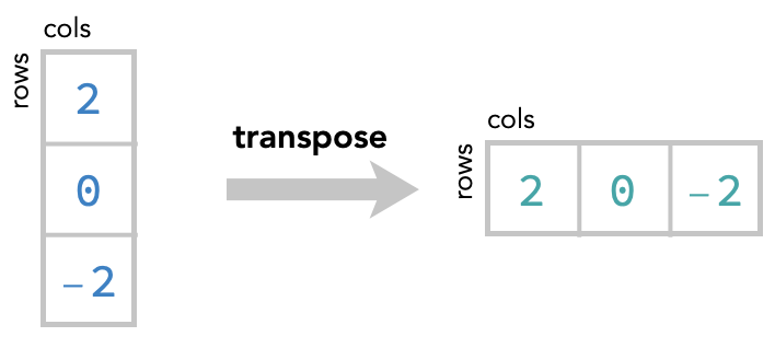
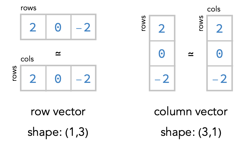
Transposing a row vector to a column vector: #

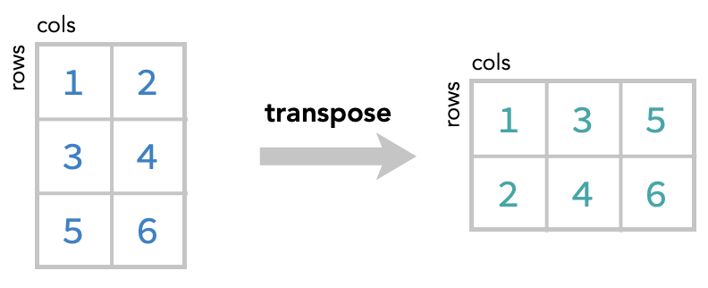
Transposing a matrix: #

Combining arrays #

Elementwise operations #

If we have multiple arrays of the same shape, it is possible to combine them as if they were numbers. For example, we can add two arrays, or multiply them, or subtract them. The way we do this is very straightforward: we simply add the ordinary numbers in the corresponding cells. This is called an elementwise operation, since it is matches elements of each array with each-other.

We’ll illustrate this with two vectors. We’ll think of these as column vectors. All this means is that we are thinking of the vector as being a column of numbers, meaning that each cell is in a different row. This intepretation isn’t part of numpy, or part of the code at all, but it is a helpful interpretation for us as humans, since it allows us to draw the vector in two dimensions, in a square diagram:

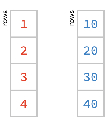
Here is the numpy code that creates these two vectors, which we’ll name r (for red) and b (for blue). Run this code:

r = np.array([1, 2, 3, 4])
b = np.array([10, 20, 30, 40])
print(r.shape, b.shape)

Notice that both vectors have the same shape, which is a 1-tuple containing 4, since there is a single axis with 4 cells in it.

We can add these two vectors by simply adding the numbers in the corresponding cells, as follows:

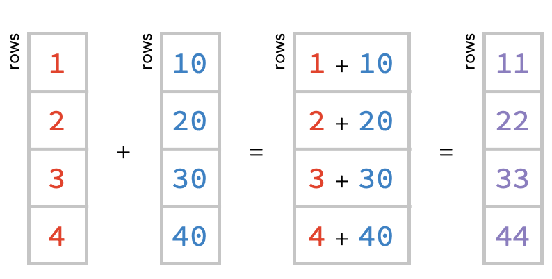
r = np.array([1, 2, 3, 4])
b = np.array([10, 20, 30, 40])
r + b

array([11, 22, 33, 44])

Task: Modify the code below to subtract 1/10 of the b vector from the a vector. What will you get?

r + b

Combining matrices #

We can also combine two matrices. Let’s again create an rm matrix and bm matrix corresponding to these:

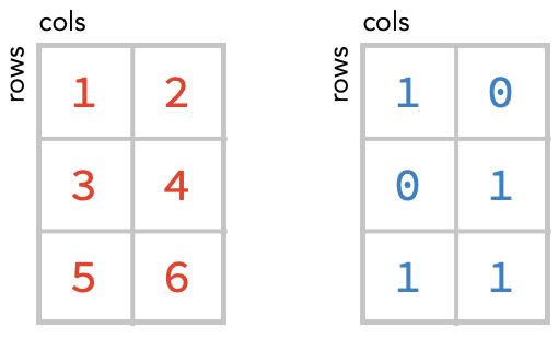
rm = np.array([[1, 2], [3, 4]])
bm = np.array([[1, 0], [0, 1]])
print(rm.shape, bm.shape)

Addition again works elementwise:

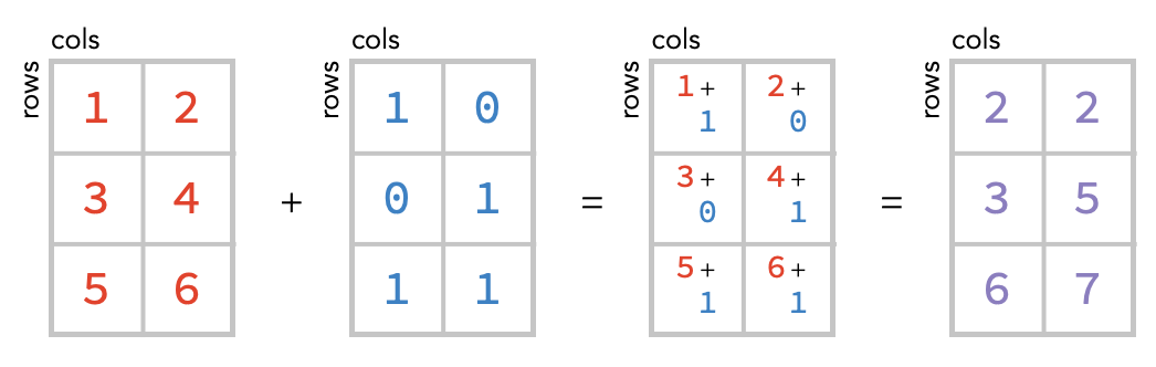
Task: Modify the code below to add the rm matrix to the bm matrix:

r + b

Broadcasting #

Interestingly, however, we can combine arrays that do not have exactly the same shape. This is easiest to explain visually.

Here’s the basic concept, which we will shortly explain:

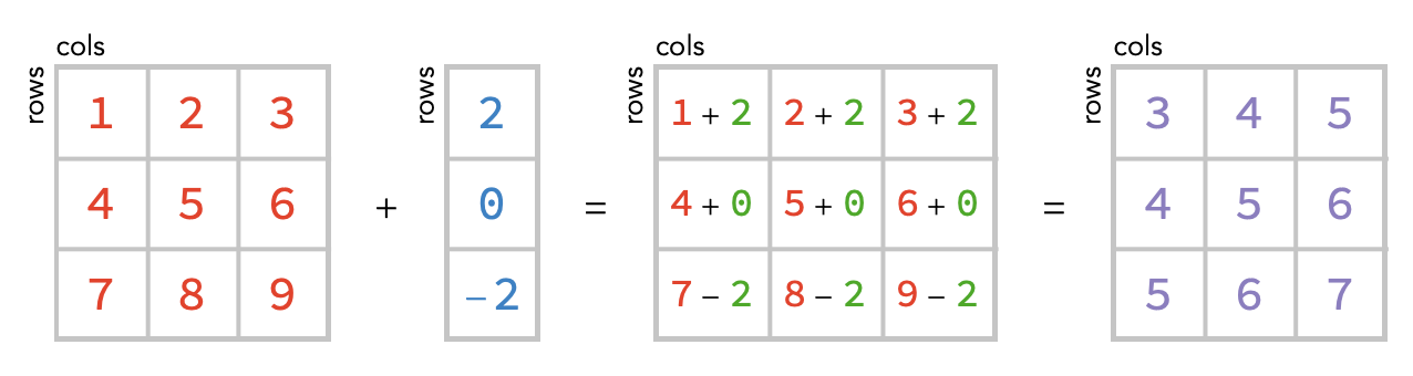
Notice the red matrix has both a row and column axis, but the blue vector only has a row axis. It is missing a column axis. So how do we match up the cells of the two arrays? The solution is simple: we treat the blue array as unchanging across these columns, so we can simply repeat the value it has in a given row – these repeated values as shown above in green.

In other words, we have made the following change when evaluating the sum:

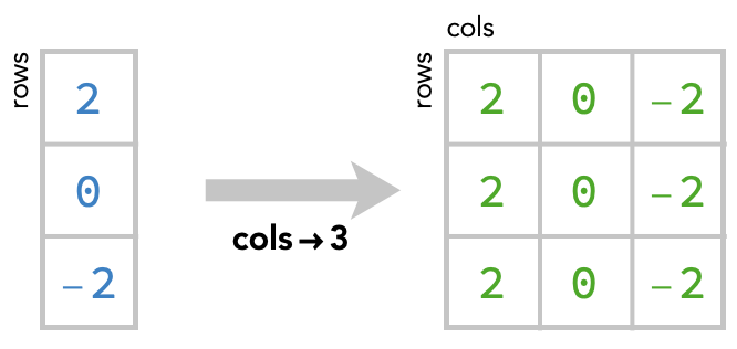
This kind of operation, in which we fill in missing axes by simply repeating the values of cells, is know broadcasting. Here’s the broadcast operation depicted on its own, where we broadcast to create a new axis with size 3, turning the vector into a matrix:

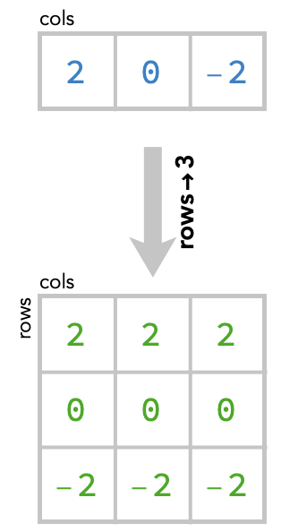
But notice there is a second way we could broadcast a vector to form a matrix:

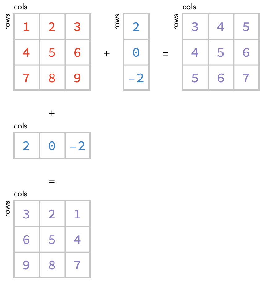
If we use this second way, then the sum would come out differently:

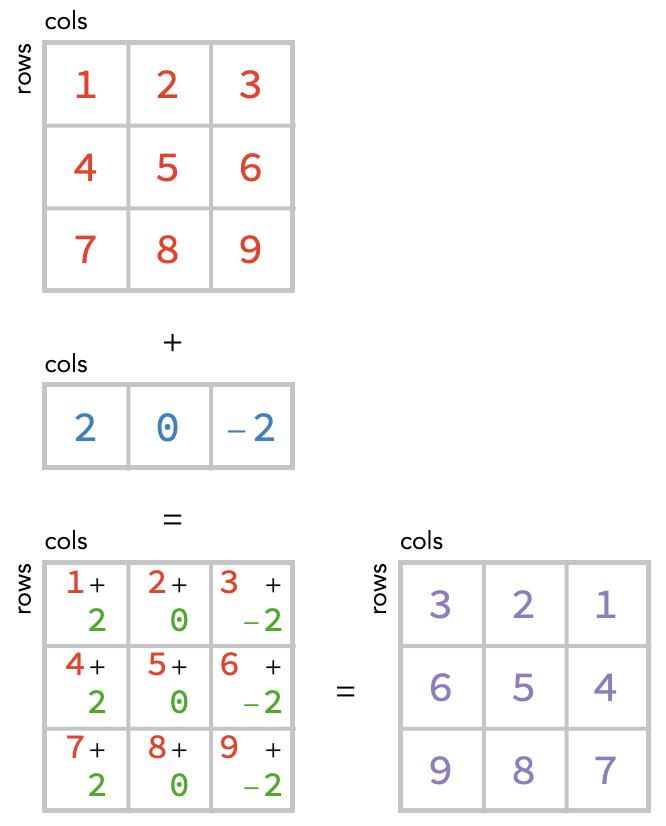
How are we to decide between these two possibilities, which we show again below?

The answer is that we have to tell numpy whether we want to consider a vector as a column vector or a row vector. We do this by taking the 1-array, which has only 1 axis (“rows”), and inserting a new axis either before or after the existing axis: There are two ways we can then do this:

Aggregating arrays #

We’ve seen that transposing retains the number of axes and cells of an array, but re-orders them. The operation of slicing can reduce the number of axes, depending on whether we select a single index (using a number like 1) or a subset of indices (using a range specification like 1:5).

The next operation we’ll consider is aggregation, which always reduces the number of axes.

Aggregation is the process of removing axes of an array by using an aggregation function that can turn multiple values into a single value. A very common and useful example of an aggregation function is sum, which takes a list of values and returns their sum. sum is built-in to Python:

sum([1,2,3,4,5])

Another useful example is max, which gives the largest out of all the values in the list:

max([1,2,3,4,5])

In general, all aggregation functions take a collection of inputs of some kind and produce a single output. But there are different ways to apply an aggregation function to an array.

For example, let’s take the following matrix:

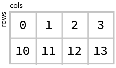
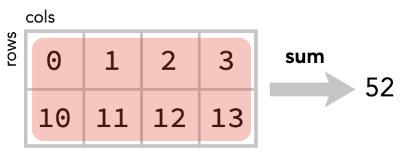
We could sum together all values of this matrix, producing a single number:

matrix = np.array([[0, 1, 2, 3], [10, 11, 12, 13]])
matrix.sum()

Here we highlight all the cells that are summed together to produce this value:

Summing across rows #

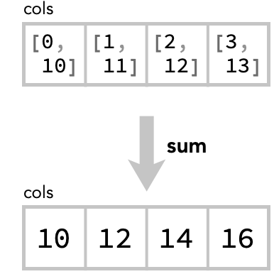
Alternatively, we could “sum across rows” – this is the operation of summing the contents of each column of the matrix. There are 4 columns so there will be 4 cells in the result of this summation:

matrix.sum(axis=0)

array([10, 12, 14, 16])

Here is the diagram of this operation:

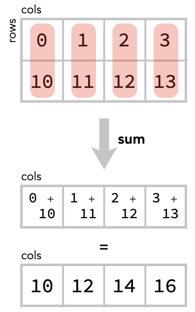
An alternative way to think about this is that we are taking the elementwise sum of two row vectors. There are two rows so we are summing two vectors, each of size 4:

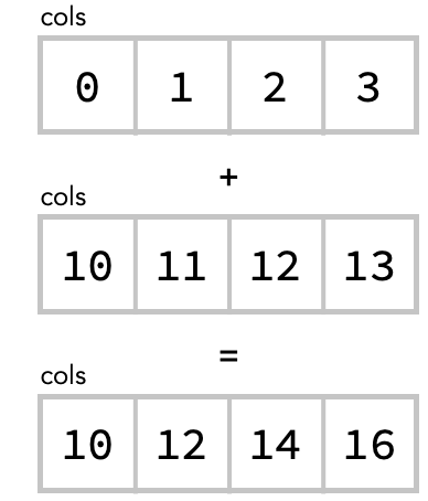
Notice that once we have “summed along rows” the row axis is gone from the result.

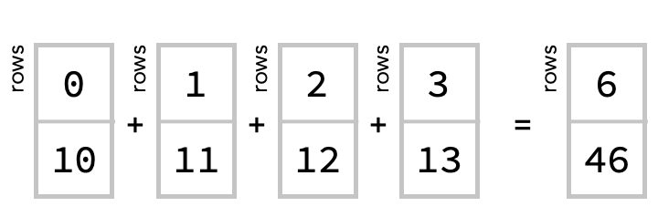
Summing across columns #

Secondly, we could “sum across columns” – which sums together the contents of each row of the matrix. There are 2 rows so there will be 2 cells in the result:

matrix.sum(axis=1)

array([ 6, 46])

Here is the diagram of this operation:

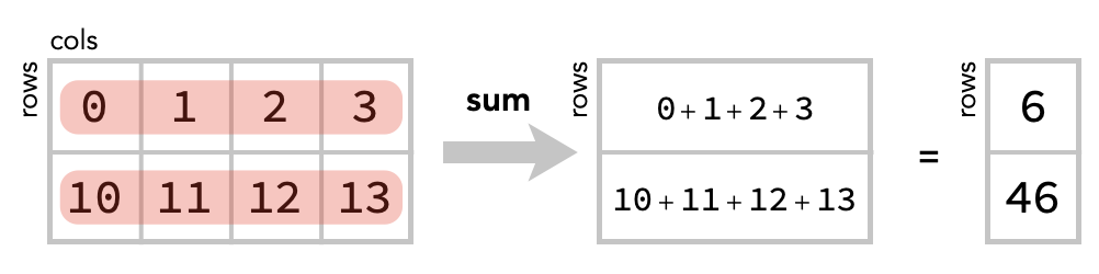
Again, we can also see this as summing four column vectors elementwise:

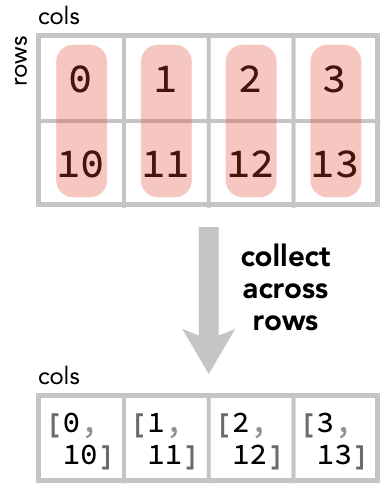
Collecting and applying #

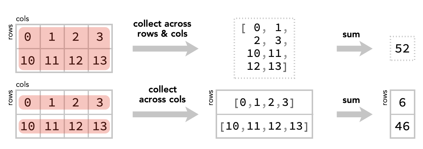
How should we think about these operations in a way that generalizes to higher order arrays?

In each of these cases, we are forming collections of cells, then feeding each collection to the aggregation function sum. The function sum is run once for each such collection, and produces a result that goes in a cell of the new array.

This suggests a general way to conceptualize aggregation: an aggregation consists of collect step and an apply step.

In the collect step, we form make a new array whose cells correspond to collections of cells from the original array. This collected array will always have a shape with fewer axes than the original array – those axes we collect are now “within” each cell.

In this example, we collect across rows / within columns, so the resulting collected array doesn’t have a rows axis:

In the apply step, we apply the chosen aggregation function (sum) to the collected values in each cell, and obtain an array of the same shape:

Let’s see this in action for the other two summations:

Notice an important, although obvious, fact: we first sum rows and then columns, or first columns and then rows, we still get the total scalar sum:

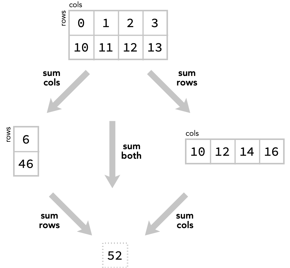
We’ll illustrate this fact by taking the original array, and summing its columns to produce a new array, and then summing the rows of that array:

summed = matrix.sum(axis=1)
print("first sum cols: ", summed)

summed = summed.sum(axis=0)
print("then sum rows: ", summed)

Task: modify the following code to do this sum the other way around: first summing the rows and then summing the columns of that result. Hint: the obvious change won’t work. Why not?

summed = matrix.sum(axis=0)
print("first sum rows: ", summed)

summed = summed.sum(axis=1)
print("then sum cols: ", summed)